Here’s a link to the live visualization. And good news: this tutorial involves no coding!

Background

More soon. For now, you can learn about MindRider helmet and data at their respective web sites.

Getting Started

1. Download QGIS and install (from QGIS) the QGIS2threejs plugin.
2. Obtain this tutorial’s data, which includes these vector shapefiles:
   • a MindRider sample dataset (800 points)
   • Manhattan’s buildings south of 14th street
   • the polygon I drew to clip the original NYC building footprints to just this region. Rendering all the buildings for the entire city could crash your browser.
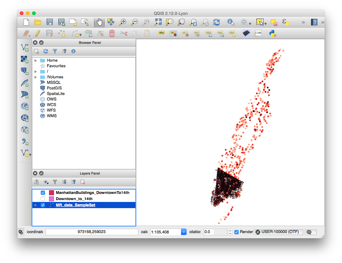
3. In QGIS, add the MindRider data by navigating to Layer > AddLayer > Add Vector Layer. Add “MR_data_SampleSet.shp” from your tutorial data.
4. NOTE: In your tutorial data folder, you’ll only be loading the shapefiles (.SHP extension). The other files (i.e. dbf, shx, etc) are supporting metadata for the shapefiles, so don’t remove them!
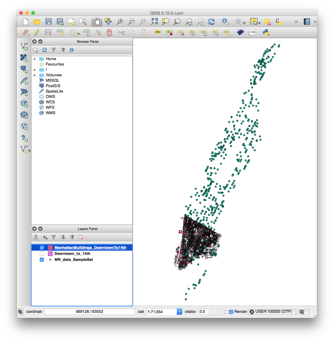
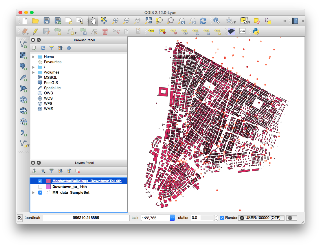
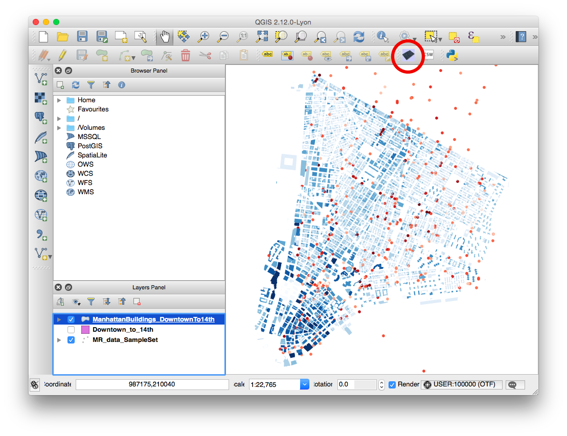
5. Add the building by navigating to Layer > AddLayer > Add Vector Layer. Add “ManhattanBuildings_DowntownTo14th.shp” from your tutorial data. Your QGIS window should now look like this:
   
6. NOTE: You can optionally add “Downtown_to_14th.shp” to your project to see what it looks like, but you won’t visualize it for the final render. If you’d like to crop another part of the building elevation data for your own purposes, see this link about creating polygons and this link about cropping shapefiles.
7. NOTE: If you import the NYC Building Data directly from its source, you will need to re-project it. See this link for a note on the proper projection to use.

Coloring the MindRider data

In this section, we will color the MindRider data points varying levels of red based on the cyclist’s mental attention, from a range of 1-100.

1. In the Layers Panel, right-click MR_data_SampleSet and choose “Properties“.
   
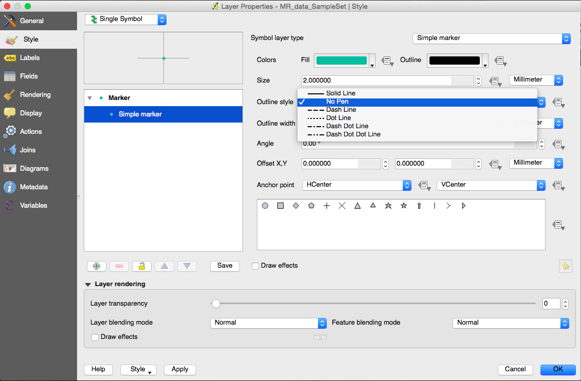
2. By default, the Properties window will be in the Style tab, and your marker type will be a Simple Marker. Remove the black outline from the markers by choosing No Pen from the Outline Style menu.
   
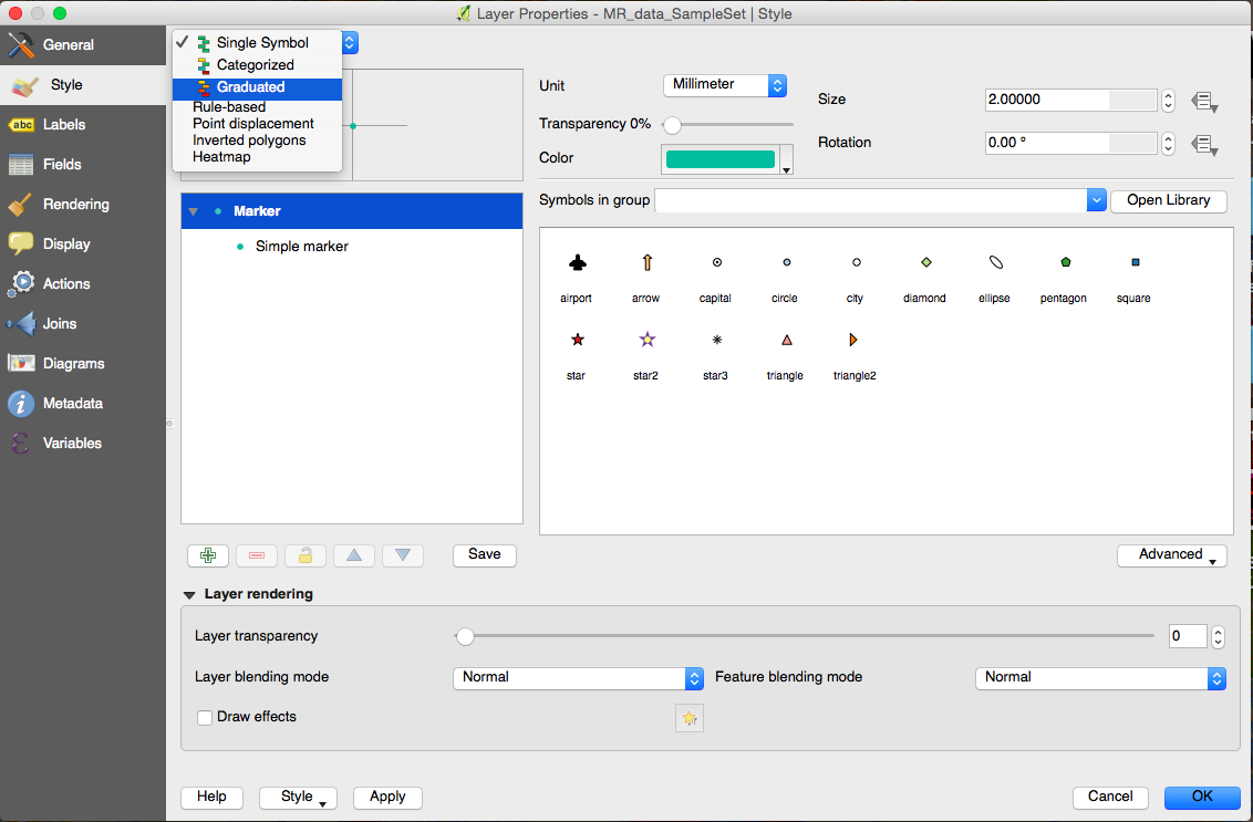
3. Next, switch from “Single Symbol” to “Graduated Symbol” in the topmost menu.
   
4.  Now change the following values:
   • COLUMN: eSenseAtte
   • COLOR RAMP: Reds
   • Classes: 100
     
     
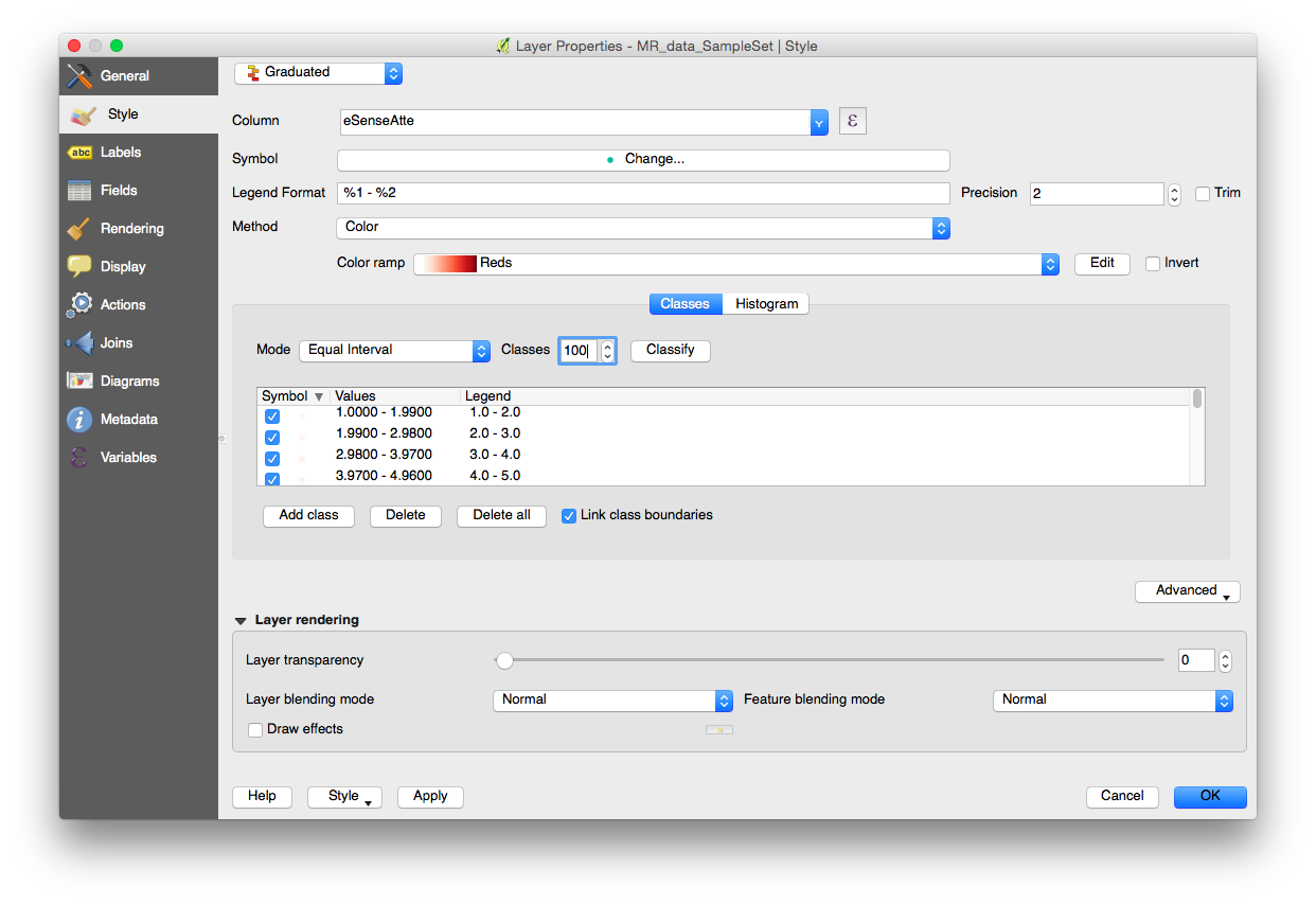
5. Press OK, and the MindRider data should now be colored according to attention values.
   

Coloring the NYC building data

You don’t need to color the buildings according to height in order to extrude them with QGIS2threejs, but after an initial attempt without the color coding, I found it color to be a helpful aid in comprehending the visualization. I chose blue to contrast with the MindRider data, which is generally colored red-yellow-green.

1. In the Layers Panel, right-click ManhattanBuildings_Downtown_to_14th and choose “Zoom to Layer.”
   
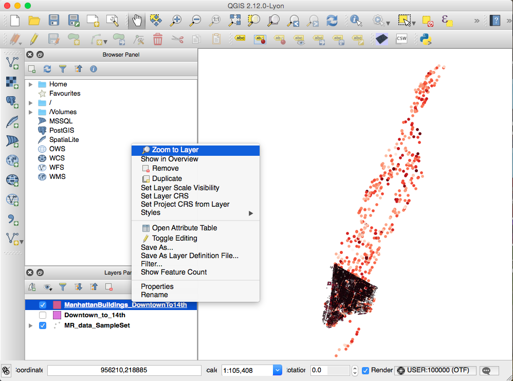
   Now you can see the layer more closely.
   
2. Remove building footprint outlines using a similar method as used for the MindRider data:
   • In the Layers Panel, right-click ManhattanBuildings_Downtown_to_14th and choose “Properties“.
   • Remove the outline by choosing Simple Marker, then choose “No Pen” in the Border Style menu.
3. Color the data a varying range by choosing Graduated in the top menu (just like you did with the MindRider data). Change these values:
   • Column: HEIGHT_ROO
   • Color Ramp: Blues
   • Mode: Natural Breaks (Jenks)
   • Classes: 10
   • 
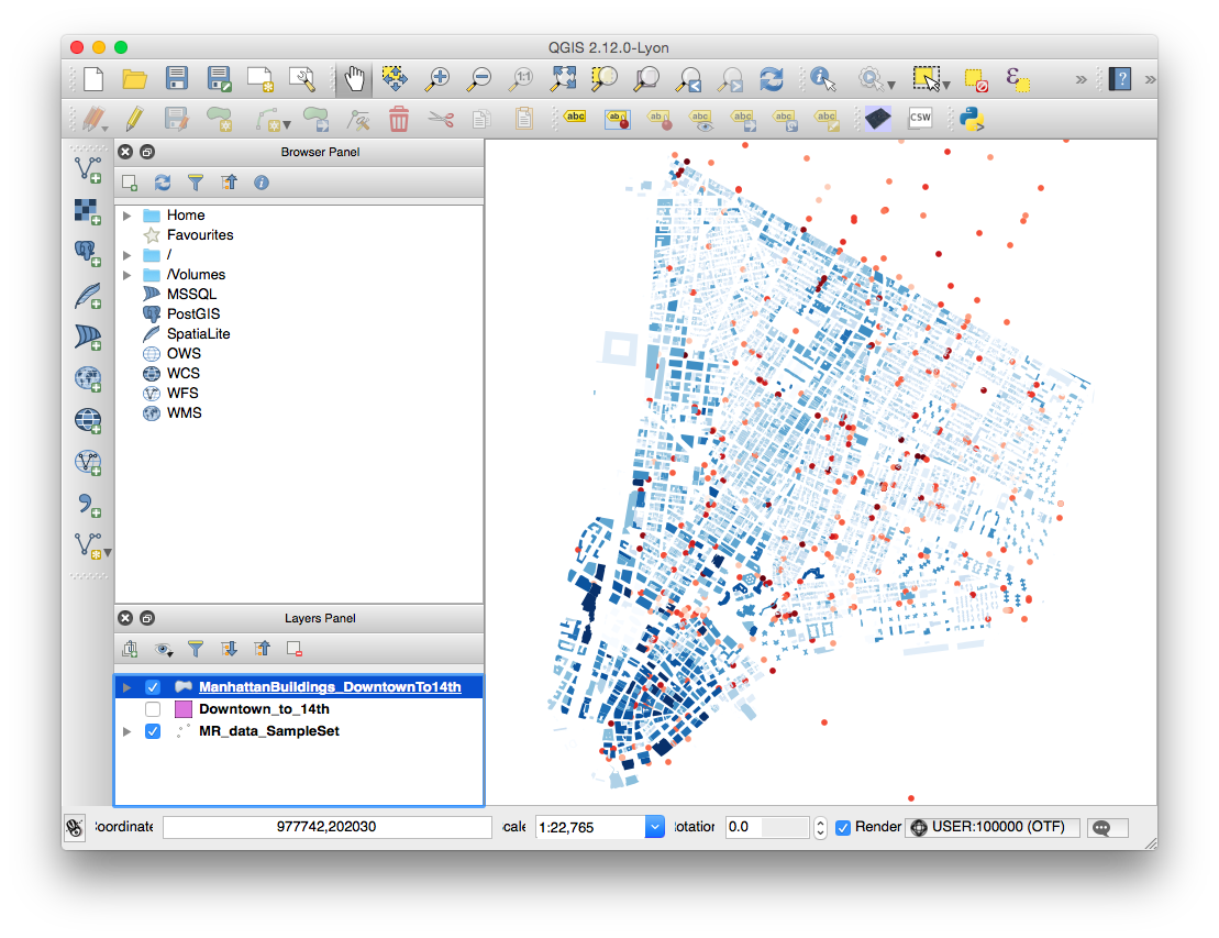
4. Press OK and see that the building data is color-coded.
   

Export (render) the data using QGIS2threejs

Let’s try exporting this data to an HTML site.

1. If you’ve installed QGIS2threejs, an icon for the plugin will show on the 2nd tier of tools in your window:
   
2. NOTE: You will only choose the ManhattanBuildings for rendering via three.js. The MindRider data, since it’s visible in the QGIS project window, will be rasterized and displayed on a flat pane at the base of the extruded buildings. If you were to render the MindRider data as 3D objects, this would make your page take a LOT longer to load.
3. In the QGIS2threejs dialog box, you only need to do two things.
   • check the box next to the ManhattanBuildings_Downtown_to_14th data set so that it will be rendered in WebGL.
   • specify Height as “HEIGHT_ROO” so that the buildings are extruded based on height.
   • 
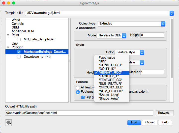
4. Specify the output file name and filepath. I recommend that you create a new directory for your file, as several supporting files will be generated in addition to the HTML file.
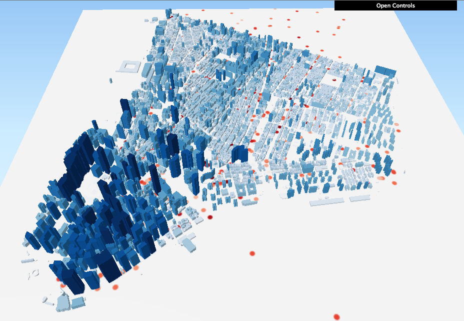
5. I called my file “test.html.” When I opened it in my browser, it looked pretty good!
   

Now for a Challenge!

You’ll notice that the image at the top of this tutorial shows both green dots and red dots, which indicate MindRider “sweetspots” (areas of high relaxation) as well as “hotspots” (areas of high attention). You’ve already visualized the hotspots. Can you visualize the sweetspots as well, and make it so that the hotspots and sweetspots blend together?

It’s pretty straightforward if you think about it. Here are the basic steps:

1. Duplicate the MR_data_SampleSet layer. Call it something like MR_sweetspots. For clarity’s sake, re-name your original MR_data_SampleSet to MR_hotspots.
2. Re-color the MR_sweetspots with a green gradient.
3. In the same dialog box where you change the layer’s color, you can experiment with Layer Rendering:
   • Try changing the layer’s transparency to 70%.
   • Try changing the layer’s blend mode to Darken or Multiply.

And see what happens! You can see my version of the sweetspots AND hotspots visualization here.